Feel Calculus With Your Programming Sense

I believe people who can code — have the ability to understand more complicated concepts than calculus. One reason why there are many talented programmers out there who are still struggling with calculus is not that it is hard. It is mostly because we have been taught it in the wrong way (along with many other topics).

If you have done some coding in your life — even some toy exercises like generating prime numbers, you might have already done similar things that happen in calculus but never had the chance to relate.

The objective of this writing is neither to teach you calculus nor programming — but to help you connect some dots.

I will get to the coding part in a minute. But allow me to give some quick background before that.

Rate of Change

Differential calculus talks about the “rate of change”. Let’s try to understand what that means.

For a change in a variable (x), the rate of change of a function is simply the change in the function divided by the change in x. Let visualize with actual numbers:

Consider 2 points x=2 and x=6, and a function y=f(x) = x².

Also, consider dx = distance between these 2 points in x-axis. And dy is the distance between y values for these x values.

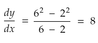
Then, the rate of change in y from x=2 to x=6 is

Derivative

Now — derivative dy/dx is the rate of change in y for an infinitesimally small change in x. Since this distance (6–2=4) is not infinitesimally small — not even close, we cannot call the above equation a derivative. So, let’s pick a smaller number, 0.1, for now.

When x = 0, y = x² = 0² = 0.

Nearest neighbour to the positive direction, x = 0.1. There y becomes 0.1² = 0.01.

So,

Let’s try one more time. Nearest neighbour of 0.1 to the positive direction, x = 0.2. So, y becomes 0.2² = 0.04. So,

If we repeat the process a few more times, this is what we get:

Here is the excel file if you wish to play with it.

dx (which is our fictional infinitesimally small distance between 2 adjacent points on the x-axis) is 0.1 in our context.

x is increasing accordingly.

y is simply x².

dy is the distance between 2 adjacent y values. For example, when x= 0.1, the distance between current y (0.01 ) and the next y (0.04) is 0.03 — so, dy is 0.03 at x=0.1.

dy/dx is dy divided by dx.

dy/dx / x is dy/dx divided by x.

Now notice that, as x increases, the last row is approaching 2, which means — the rate of change of x² with respect to x is approaching twice of x, which is 2x.

Remember the derivative of x² with respect to x? 2x! Finding some connection?

Coding Time

Let’s try the things in code that we have been discussing so far.

Assuming you already have Python installed, in the terminal, run:

After that, run the following Python code:

Here:

x: containing numbers from 0 to 9.

y: another array, each element is square of corresponding x element

dy: Another array initialized with zeros. We will put y-distances in this array.

dydx: Another array initialized with zeros. It will contain the dy/dx value of every point.

dx: Pretty obvious — it is the step size. Distance between 2 consecutive numbers, which decreases as SIZE increases. If SIZE = 10, dx = 1. If SIZE = 100, dx = 0.1.

First, we are deriving dy for every point. Then we calculate dydx from it.

Notice that:

Here we are omitting the first and last values. The first value of x is 0, which will produce a zero-division error. And we cannot calculate the last value of dy/dx since we do not have the last value of dy — because it would require next to the last available value of y, which we don’t have here.

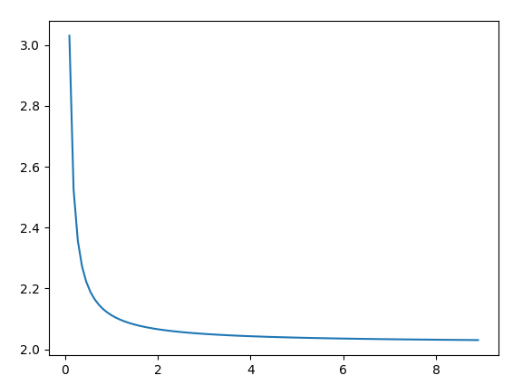
If everything goes fine, you will get this graph:

What you understand from the plot

As you see, the graph is approaching 2. Increase the value of SIZE (meaning setting lower of dx) and see how the graph more quickly approaches 2.

Second Derivative

Now that you have come this far, just a few more steps to realize the second derivative, which will give you the intuition for derivative of any order.

As you remember, the second derivative is the rate of change of the first derivative with respect to x. Simply put — dy/dx in the second derivative is like y in the first derivative.

Let’s do the following modifications to the code above:

Declare 2 more arrays:

d2ydx2: Which will represent the second derivative:

distance_dydx: To represent distance between dy/dx value between 2 adjacent points

Here is the full code for the second derivative:

After calculating dydx in the for loop, we execute another loop to calculate the second derivative. With some wise coding, we could calculate the second derivative in the same loop (try as an exercise) —but I kept them separate here for clarity.

Also, notice that:

As we did in the first derivative, we are omitting some values here as well. The last 2 values are omitted since the second from the last would require the last “first derivative” value, which we couldn’t calculate (since we didn’t have the required y value for it — as described above). Does it mean we have to omit the last 3 values in the case of 3rd derivative?🤔 — that is for you to find.

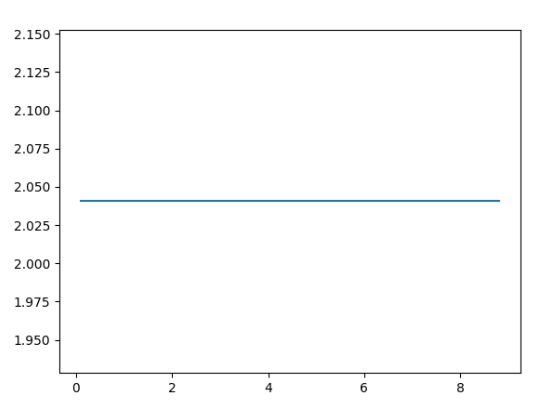
Here is the output graph:

What do we see here?

As you know from high school:

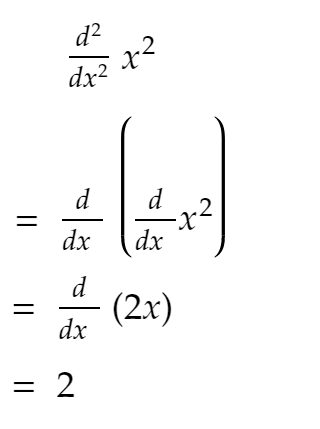
Now, as you see from the code above, the second derivative mostly remains constant, and if you keep increasing SIZE — it approaches 2!

Why rate of change is important

You might be wondering:

— Why do we get through all these nasty troubles? What useful information do we get from the rate of change or derivative?

— Why can’t we just go with the rate of change for any amount? Why only infinitesimally small? What information do we get from the change rate with respect to infinitesimally small, which cannot be found from the rate of change with respect to bigger values?

— This infinitesimally small thing kind of looks like a hack? We worked with some small numbers above alright — but surely not actually infinitesimally small.

If I allow myself to keep going, you would walk away seeing the length of this article and wouldn’t have come this far. Maybe we will address those questions some other day 😀.