Single Neuron Neural Network on Python – With Mathematical Intuition

Let’s build a simple network — very very simple, but a complete network – with a single layer. Only one input — and one neuron (which is the output as well), one weight, one bias.

Let’s run the code first and then analyze part by part

Clone the Github project, or simply run the following code in your favorite IDE.

If you need help in setting up an IDE, I described the process here.

If everything goes okay, you will get this output:

The Problem — Fahrenheit from Celsius

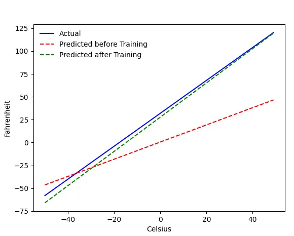
We will train our machine to predict Fahrenheit from Celsius. As you can understand from the code (or the graph), the blue line is the actual Celsius-Fahrenheit relation. The red line is the relation predicted by our baby machine without any training. Finally, we train the machine, and the green line is the prediction after training.

Look at Line#65–67 — before and after training, it is predicting using the same function (get_predicted_fahrenheit_values()). So what magic train() is doing? Let’s find out.

Network Structure

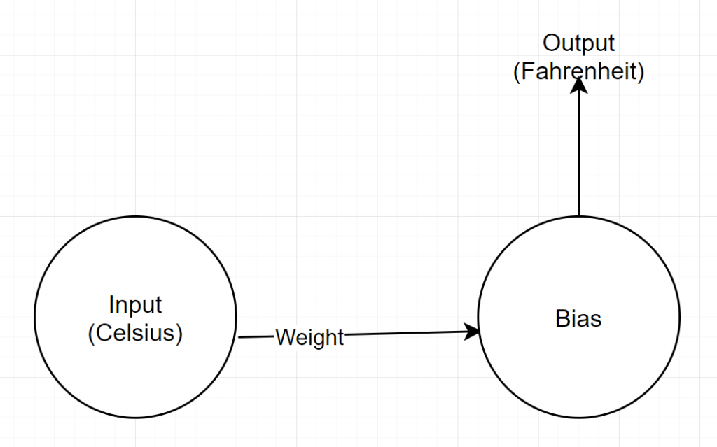
Input: A number representing celsius

Weight: A float representing the weight

Bias: A float representing bias

Output: A float representing predicted Fahrenheit

So, we have total 2 parameters — 1 weight and 1 bias

Code Analysis

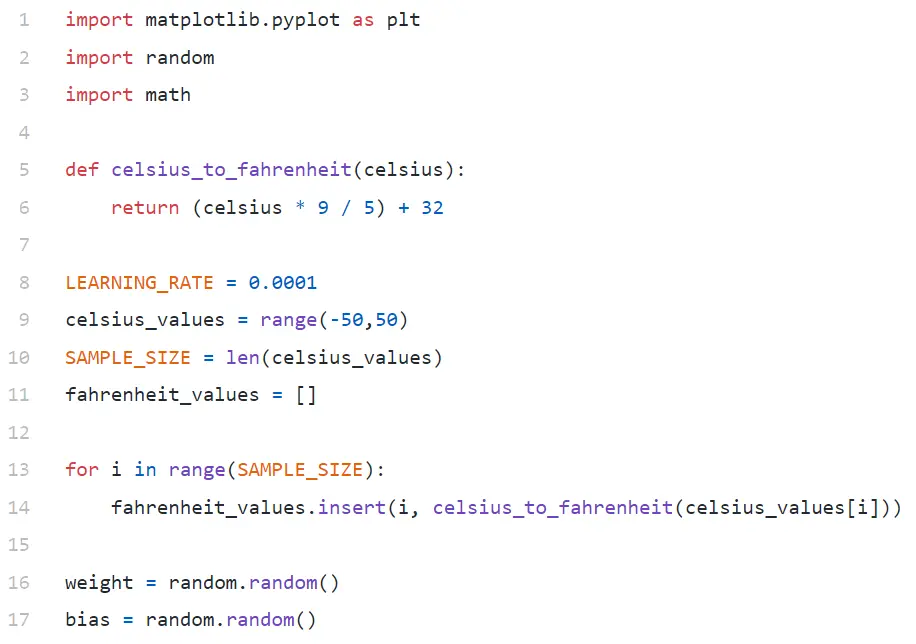
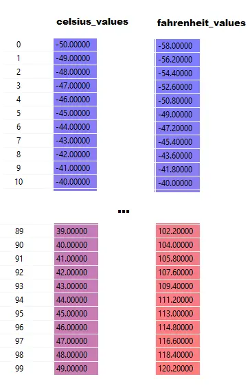
In Line#9, we are generating an array of 100 numbers between -50 and +50 (excluding 50 — range function excludes the upper limit value).

In Line#11–14, we are generating the Fahrenheit for each celsius value.

In line#16 and #17, we are initializing weight and bias.

train()

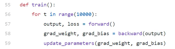
We are running 10000 iterations of training here. Each iteration is made of:

1. forward (Line#57) pass
2. backward (Line#58) pass
3. update_parameters (Line#59)

If you are new to python, it might look a bit strange to you — python functions can return multiple values as tuple.

Notice that update_parameters is the only thing we are interested in. Everything else we are doing here is to evaluate the parameters of this function, which are the gradients (we will explain below what gradients are) of our weight and bias.

1. grad_weight: A float representing gradient of weight
2. grad_bias: A float representing gradient of bias

We get these values by calling backward, but it requires output, which we get by calling forward at line#57.

forward()

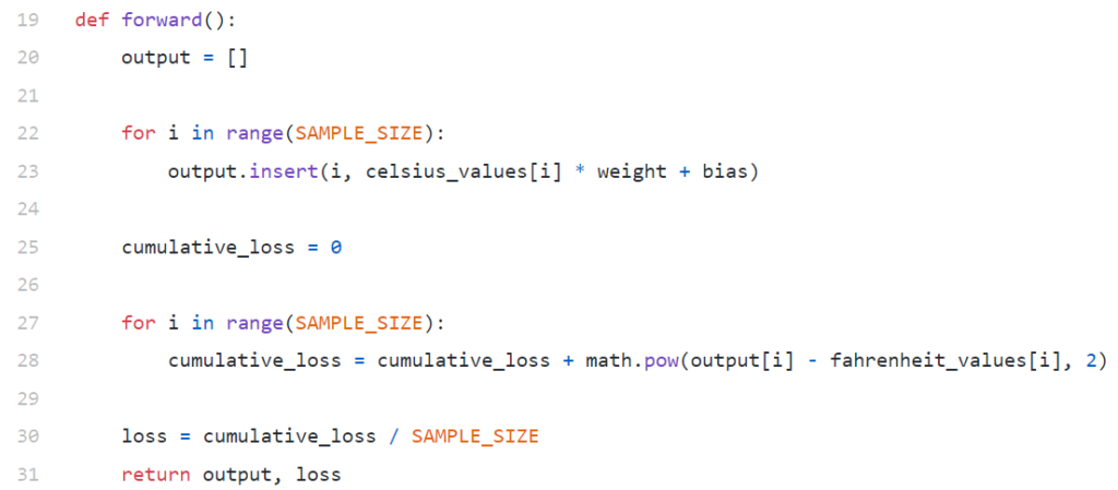
Notice that here celsius_values and fahrenheit_values are arrays of 100 rows:

After executing Line#20–23, for a celsius value, say 42

output =42 * weight + bias

So, for 100 elements in celsius_values, output will be array of 100 elements for each corresponding celsius value.

Line#25–30 is calculating loss using Mean Squared Error (MSE) loss function, which is just a fancy name of the square of all differences divided by the number of samples (100 in this case).

Small loss means better prediction. If you keep printing loss in every iteration, you will see that it is decreasing as training progresses.

Finally, in Line#31 we are returning predicted output and loss.

backward

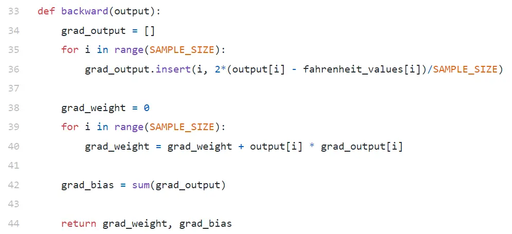
We are only interested to update our weight and bias. To update those values, we have to know their gradients, and that is what we are calculating here.

Notice gradients are being calculated in reverse order. Gradient of output is being calculated first, and then for weight and bias, and so the name “backpropagation”. The reason is, to calculate gradient of weight and bias, we need to know gradient of output — so that we can use it in the chain rule formula.

Now let’s have a look at what gradient and chain rule are.

Gradient

For the sake of simplicity, consider we have only one value of celsius_values and fahrenheit_values, 42 and 107.6 respectively.

Now, the breakdown of the calculation in Line#30 becomes:

loss = (107.6 — (42 * weight + bias))² / 1

As you see, loss depends on 2 parameters — weights and bias. Consider the weight. Imagine, we initialized it with a random value, say, 0.8, and after evaluating the equation above, we get 123.45 as the value of loss. Based on this loss value, you have to decide how you will update weight. Should you make it 0.9, or 0.7?

You have to update weight in a way so that in the next iteration you get a lower value for loss (remember, minimizing loss is the ultimate goal). So, if increasing weight increases loss, we will decrease it. And if increasing weight decreases loss, we will increase it.

Now, the question, how we know if increasing weights will increase or decrease loss. This is where the gradient comes in. Broadly speaking, gradient is defined by derivative. Remember from your high school calculus, ∂y/∂x (which is partial derivative/gradient of y with respect to x) indicates how y will change with a small change in x.

If ∂y/∂x is positive, it means a small increment in x will increase y.

If ∂y/∂x is negative, it means a small increment in x will decrease y.

If ∂y/∂x is big, a small change in x will cause a big change in y.

If ∂y/∂x is small, a small change in x will cause a small change in y.

So, from gradients, we get 2 information. Which direction the parameter has to be updated (increase or decrease) and how much (big or small).

Chain Rule

Informally speaking, the chain rule says:

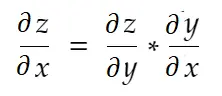
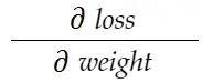
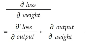
Consider example of weight above. We need to calculate grad_weight to update this weight, which will be calculated by:

With chain rule formula, we can derive it:

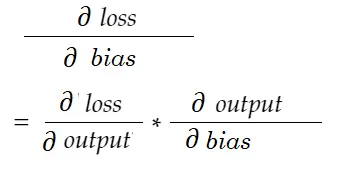
Similarly, gradient for bias:

Let’s draw a dependency diagram.

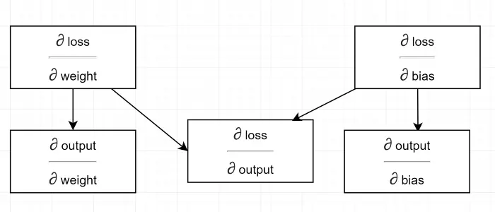
See all calculation depends on the gradient of output (∂ loss/∂ output). That is why we are calculating it first on the backpass (Line#34–36).

In fact, in high-level ML frameworks, for example in PyTorch, you don’t have to write codes for backpass! During the forward pass, it creates computational graphs, and during back pass, it goes through opposite direction in the graph and calculates gradients using chain rule.

∂ loss / ∂ output

We define this variable by grad_output in code, which we calculated in Line#34–36. Let’s find out the reason behind the formula we used in the code.

Remember, we are feeding all 100 celsius_values in the machine together. So, grad_output will be an array of 100 elements, each element containing gradient of output for the corresponding element in celsius_values. For simplicity, let us consider, there are only 2 items in celsius_values.

So, breaking down line#30,

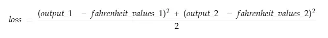
where,

output_1 = output value for 1st celsius value

output_2 = output value for 2nd celsius value

fahreinheit_values_1 = Actual fahreinheit value for 1st celsius value

fahreinheit_values_1 = Actual fahreinheit value for 2nd celsius value

Now, the resulting variable grad_output will contain 2 values — gradient of output_1 and output_2, meaning:

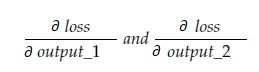
Let us calculate the gradient of output_1 only, and then we can apply the same rule for the others.

Calculus time!

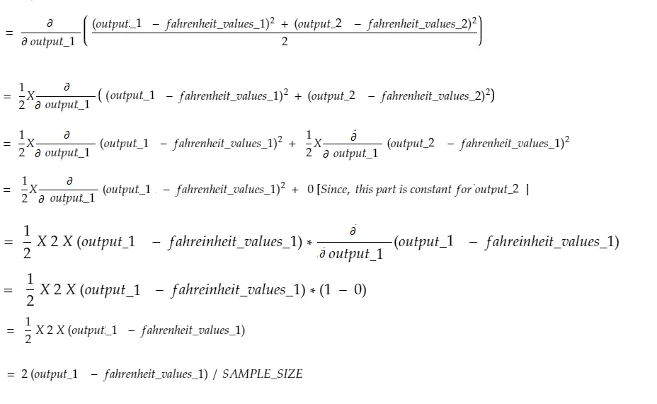
Which is the same as line#34–36.

Weight gradient

Imagine, we have only one element in celsius_values. Now:

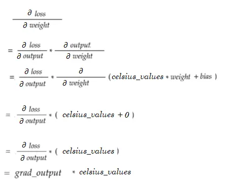
Which is same as Line#38–40. For 100 celsius_values, gradient values for each of the values will be summed up. An obvious question would be why aren’t we scaling down the result (i.e. dividing with SAMPLE_SIZE). Since we are multiplying all the gradients with a small factor before updating the parameters, it is not necessary (see the last section Updating Parameters).

Bias gradient

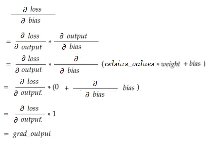
Which is same as Line#42. Like weight gradients, these values for each of the 100 inputs are being summed up. Again, it is fine since gradients are multiplied with a small factor before updating parameters.

Updating Parameters

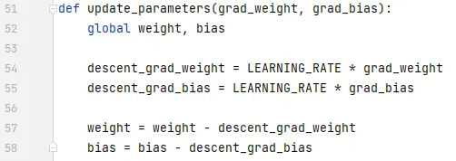
Finally, we are updating the parameters. Notice that the gradients multiplied by a small factor (LEARNING_RATE) before getting subtracted, to make the training stable. A big value of LEARNING_RATE will cause an overshooting issue and an extremely small value will make the training slower, which might need a lot more iterations. We should find an optimal value for it with some trial and error. There are many online resources on it including this one to know more about learning Rate.

Notice that, the exact amount we adjust is not extremely critical. For example, if you tune LEARNING_RATE a bit, the descent_grad_weight and descent_grad_bias variables (Line#49–50) will be changed, but the machine might still work. The important thing is making sure these amounts are derived by scaling down the gradients with the same factor (LEARNING_RATE in this case). In other words, “keeping the descent of the gradients proportional” matters more than “how much they descent”.

Also notice that these gradient values are actually sum of gradients evaluated for each of the 100 inputs. But since these are scaled with the same value, it is fine as mentioned above.

In order to update the parameters, we have to declare them with global keyword (in Line#47).

Where to go from here

The code would be much smaller by replacing the for loops with list comprehension in pythonic way. Have a look at it now — wouldn’t take more than a few minutes to understand.

If you understood everything so far, probably it is a good time to see the internals of a simple network with multiple neurons/layers — here is an article.